Department of Physics

Welcome to the Department of Physics at Durham
The Physics Department is a thriving centre for research and education.
We are proud that our Department closely aligns the teaching and learning experience for its students with the research-intensive values and practices of the University. Research-led teaching is embedded at all levels from first year laboratory reports to our final year MSci flagship individual research projects.
The Department incorporates the Ogden Centre for Fundamental Physics, is home to the Institute for Particle Physics Phenomenology and the Institute for Computational Cosmology. The Ogden Centre is also the base for our innovative outreach programme for school children and their teachers.


/prod01/prodbucket01/media/durham-university/research-/doctoral-training-centres/durham-global-challenges-centre/86240.jpg)
Just got your grades?
We look forward to welcoming you to Physics. Find out what to do next below.
What's new?
-
Working to answer the ultimate question – are we alone in the Universe?
Dr Cyril Bourgenot from our Centre for Advanced Instrumentation is part of a team developing cutting-edge technology to enable astronomers to look deeper into the Universe. He is presenting this work as part of the Royal Astronomical Society’s National Astronomy Meeting 2025, which is being hosted by Durham University this week. Here, Cyril tells us about his work and how it could help answer the ultimate astronomical question – is there life elsewhere.Global research/prod01/prodbucket01/media/durham-university/central-news-and-events-images/Updated-NAM-QA-with-Cyril---Web-.png)
-
Bright young stars light up UK's National Astronomy Meeting
Young people are at the centre of a major national conference bringing some of the world's finest scientists to the region.Durham news/prod01/prodbucket01/media/durham-university/central-news-and-events-images/news/NAM-school-events-story---Web-.jpg)
-
National Astronomy Meeting 2025 – discover our free public events
We’re celebrating our role as hosts of the UK’s leading astronomy conference next week (7-11 July) with a series of free events for the public to enjoy.Durham news/prod01/prodbucket01/media/durham-university/central-news-and-events-images/news/NAM-public-events-story---Web-.jpg)
-
National Astronomy Meeting 2025 - exploring Durham’s rich astronomical research
Almost a thousand of the world’s top space scientists will visit Durham University next week (7 to 11 July) as we host the UK’s National Astronomy Meeting (NAM) 2025.Global research/prod01/prodbucket01/media/durham-university/central-news-and-events-images/news/NAM-launch---Web-.jpg)
-
‘World-class’ research showcased during Europe-wide summit
The global impact of our research has been highlighted during a visit by the European Research Council Scientific Council.Research news/prod01/prodbucket01/media/durham-university/central-news-and-events-images/ERC-web-story.jpg)
-
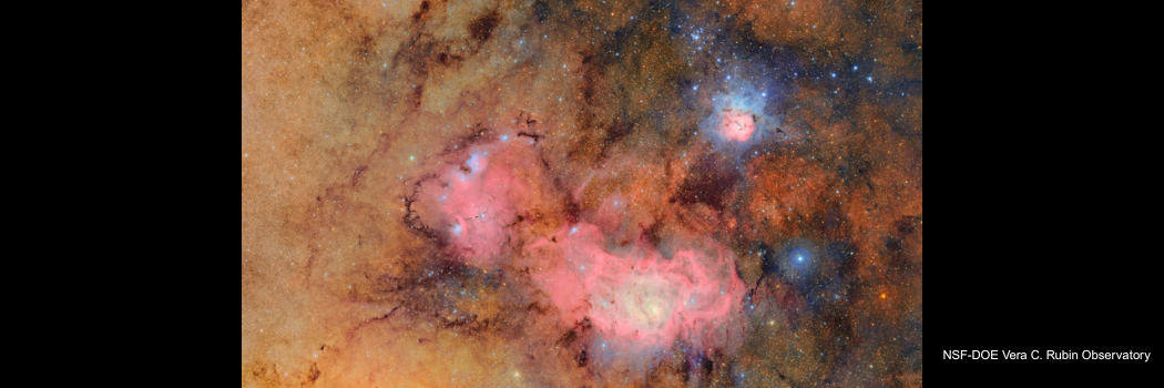
Durham scientists play key role in global space survey as first Rubin Observatory images released
Scientists from our top-rated Physics department are playing a major role in the world’s most ambitious space project, the Legacy Survey of Space and Time (LSST), led by the Vera C. Rubin Observatory.Research news/prod01/prodbucket01/media/durham-university/central-news-and-events-images/Rubin-space-WEB.png)
-
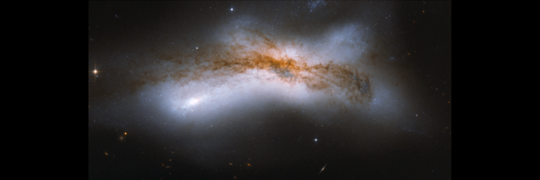
New study casts doubt on the likelihood of Milky Way collision with Andromeda
New research has cast doubt on the long-held theory that our galaxy, the Milky Way, will collide with its largest neighbour, the Andromeda galaxy, in 4.5 billion years-time.Global research/prod01/prodbucket01/media/durham-university/central-news-and-events-images/news/MW-And-collision-web-pic.png)
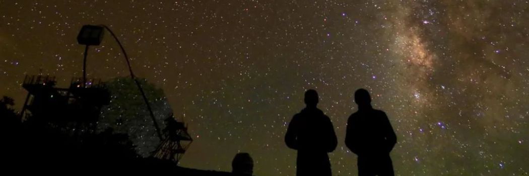
Working to answer the ultimate question – are we alone in the Universe?
Dr Cyril Bourgenot from our Centre for Advanced Instrumentation is part of a team developing cutting-edge technology to enable astronomers to look deeper into the Universe. He is presenting this work as part of the Royal Astronomical Society’s National Astronomy Meeting 2025, which is being hosted by Durham University this week. Here, Cyril tells us about his work and how it could help answer the ultimate astronomical question – is there life elsewhere.

Bright young stars light up UK's National Astronomy Meeting

National Astronomy Meeting 2025 – discover our free public events

National Astronomy Meeting 2025 - exploring Durham’s rich astronomical research
‘World-class’ research showcased during Europe-wide summit
Durham scientists play key role in global space survey as first Rubin Observatory images released
New study casts doubt on the likelihood of Milky Way collision with Andromeda
-
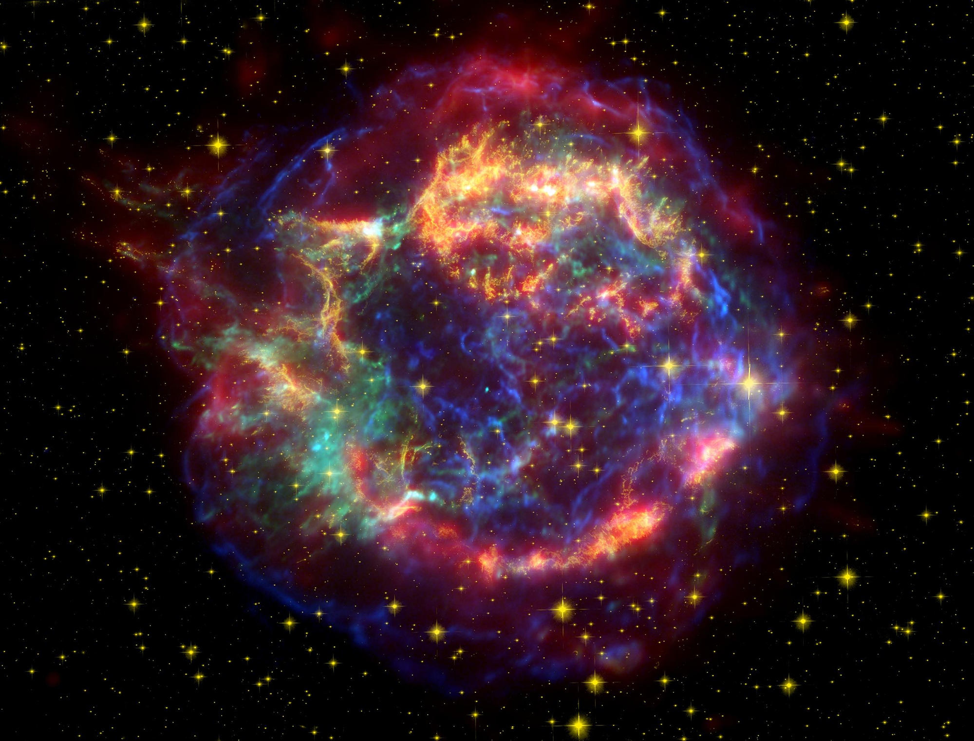
New ‘mini halo’ discovery deepens our understanding of how the early Universe was formed
Astronomers have uncovered a vast cloud of energetic particles surrounding one of the most distant galaxy clusters ever observed, marking a major step forward in understanding the hidden forces that shape the cosmos.Research news/prod01/prodbucket01/media/durham-university/central-news-and-events-images/news/Mini-halo-web-pic.png)
-
‘World-class’ research showcased during Europe-wide summit
The global impact of our research has been highlighted during a visit by the European Research Council Scientific Council.Research news
-
Durham scientists play key role in global space survey as first Rubin Observatory images released
Scientists from our top-rated Physics department are playing a major role in the world’s most ambitious space project, the Legacy Survey of Space and Time (LSST), led by the Vera C. Rubin Observatory.Research news
New ‘mini halo’ discovery deepens our understanding of how the early Universe was formed
Astronomers have uncovered a vast cloud of energetic particles surrounding one of the most distant galaxy clusters ever observed, marking a major step forward in understanding the hidden forces that shape the cosmos.

‘World-class’ research showcased during Europe-wide summit
Durham scientists play key role in global space survey as first Rubin Observatory images released
-
Bright young stars light up UK's National Astronomy Meeting
Young people are at the centre of a major national conference bringing some of the world's finest scientists to the region.Durham news
-
National Astronomy Meeting 2025 – discover our free public events
We’re celebrating our role as hosts of the UK’s leading astronomy conference next week (7-11 July) with a series of free events for the public to enjoy.Durham news
-
The Rochester Lecture 2025 will be delivered by Nobel Prize Laureate Prof. Anne L'Huillier
When an intense laser interacts with a gas of atoms, high-order harmonics are generated. In the time domain, this radiation forms a train of extremely short light pulses, of the order of 100 attoseconds. Attosecond pulses allow the study of the dynamics of electrons in atoms and molecules, using pump-probe techniques. Anne L'Huillier's lecture will highlight some of the key steps of the field of attosecond science. Her talk is titled 'The Route to Attosecond Light Pulses'.Durham news/prod01/prodbucket01/media/durham-university/departments-/physics/major-lecture-series/Anne-LHullier.jpg)
Bright young stars light up UK's National Astronomy Meeting
Young people are at the centre of a major national conference bringing some of the world's finest scientists to the region.
National Astronomy Meeting 2025 – discover our free public events
The Rochester Lecture 2025 will be delivered by Nobel Prize Laureate Prof. Anne L'Huillier
-
Working to answer the ultimate question – are we alone in the Universe?
Dr Cyril Bourgenot from our Centre for Advanced Instrumentation is part of a team developing cutting-edge technology to enable astronomers to look deeper into the Universe. He is presenting this work as part of the Royal Astronomical Society’s National Astronomy Meeting 2025, which is being hosted by Durham University this week. Here, Cyril tells us about his work and how it could help answer the ultimate astronomical question – is there life elsewhere.Global research
-
National Astronomy Meeting 2025 - exploring Durham’s rich astronomical research
Almost a thousand of the world’s top space scientists will visit Durham University next week (7 to 11 July) as we host the UK’s National Astronomy Meeting (NAM) 2025.Global research
-
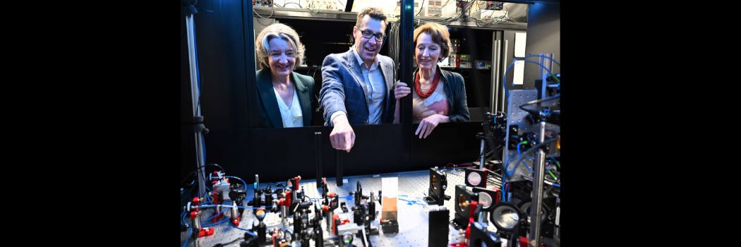
ERC Spotlight: Professor Simon Cornish and global milestones in quantum physics
We will host the European Research Council's (ERC) Scientific Council Meeting this June. Leading up to the visit, we are highlighting some of the projects at Durham that are happening thanks to support from the ERC.Global research/prod01/prodbucket01/media/durham-university/research-/ERC-Campaign---Simon-Cornish---Web-story-header.png)
Working to answer the ultimate question – are we alone in the Universe?
Dr Cyril Bourgenot from our Centre for Advanced Instrumentation is part of a team developing cutting-edge technology to enable astronomers to look deeper into the Universe. He is presenting this work as part of the Royal Astronomical Society’s National Astronomy Meeting 2025, which is being hosted by Durham University this week. Here, Cyril tells us about his work and how it could help answer the ultimate astronomical question – is there life elsewhere.
National Astronomy Meeting 2025 - exploring Durham’s rich astronomical research
ERC Spotlight: Professor Simon Cornish and global milestones in quantum physics

-
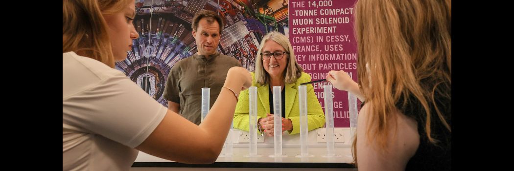
Government Minister visits Ukraine summer camp
The UK’s Higher Education Minister has visited our campus to show her support for an education and recreation summer camp for Ukrainian young people.Equality, Diversity, and Inclusion/prod01/prodbucket01/media/durham-university/central-news-and-events-images/Minister-visit-web.jpg)
-
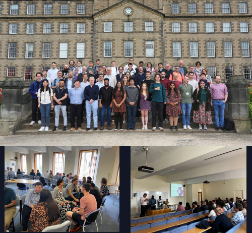
Condensed Matter Physics Research Section came together for an Away Day
The whole Condensed Matter Physics research section (CMP) in Physics at Durham came together for an Away Day at Ushaw House for training and development activities to strengthen our research capabilities and support career progression.Equality, Diversity, and Inclusion/prod01/prodbucket01/media/durham-university/departments-/physics/news-images/CMP-News-Image.jpg)
-
Celebrating the next generation of North East Physicists
Physics students’ success from across the region has been celebrated at the recent School Physicist of the Year (SPotY) awards.Equality, Diversity, and Inclusion/prod01/prodbucket01/media/durham-university/young-physicists---Website-news-article-image-(1050-x-350px)-(1).png)
Government Minister visits Ukraine summer camp
The UK’s Higher Education Minister has visited our campus to show her support for an education and recreation summer camp for Ukrainian young people.
Condensed Matter Physics Research Section came together for an Away Day
Celebrating the next generation of North East Physicists
-(1).png)
Study with us
-
Undergraduate study
Find out more about our BSc and MPhys courses.

-
Postgraduate study
Discover more about our taught courses and research degrees.
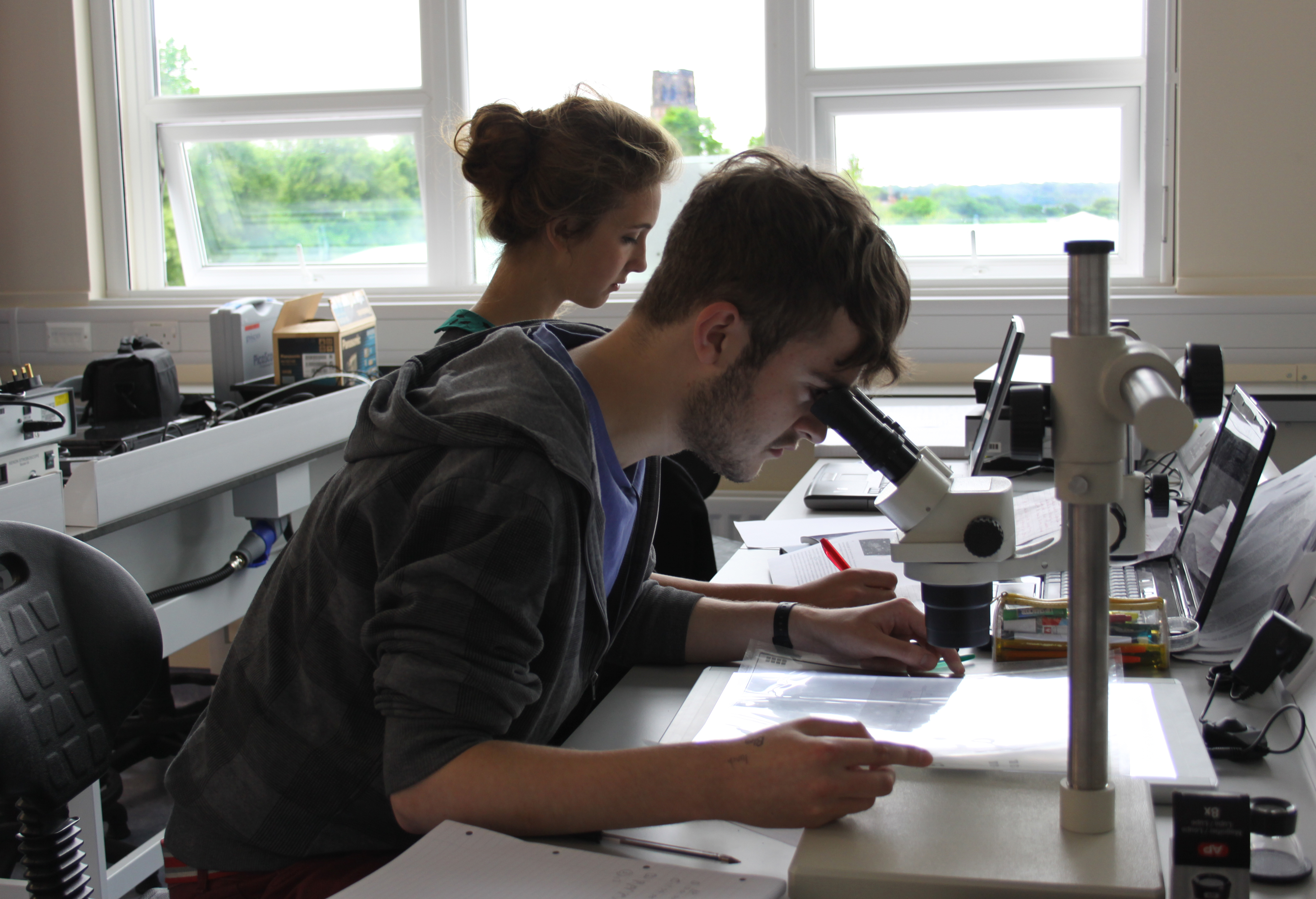
/prod01/prodbucket01/media/durham-university/departments-/physics/teaching-labs/IMG_1095.jpg)
/prod01/prodbucket01/media/durham-university/departments-/physics/postgraduates/000583826-ECR-01-3424X2714.JPG)
Undergraduate study
Find out more about our BSc and MPhys courses.
Postgraduate study
Discover more about our taught courses and research degrees.

Our research
We are one of the top Physics Departments in the UK for research, as recognised in repeated assessments and league tables.
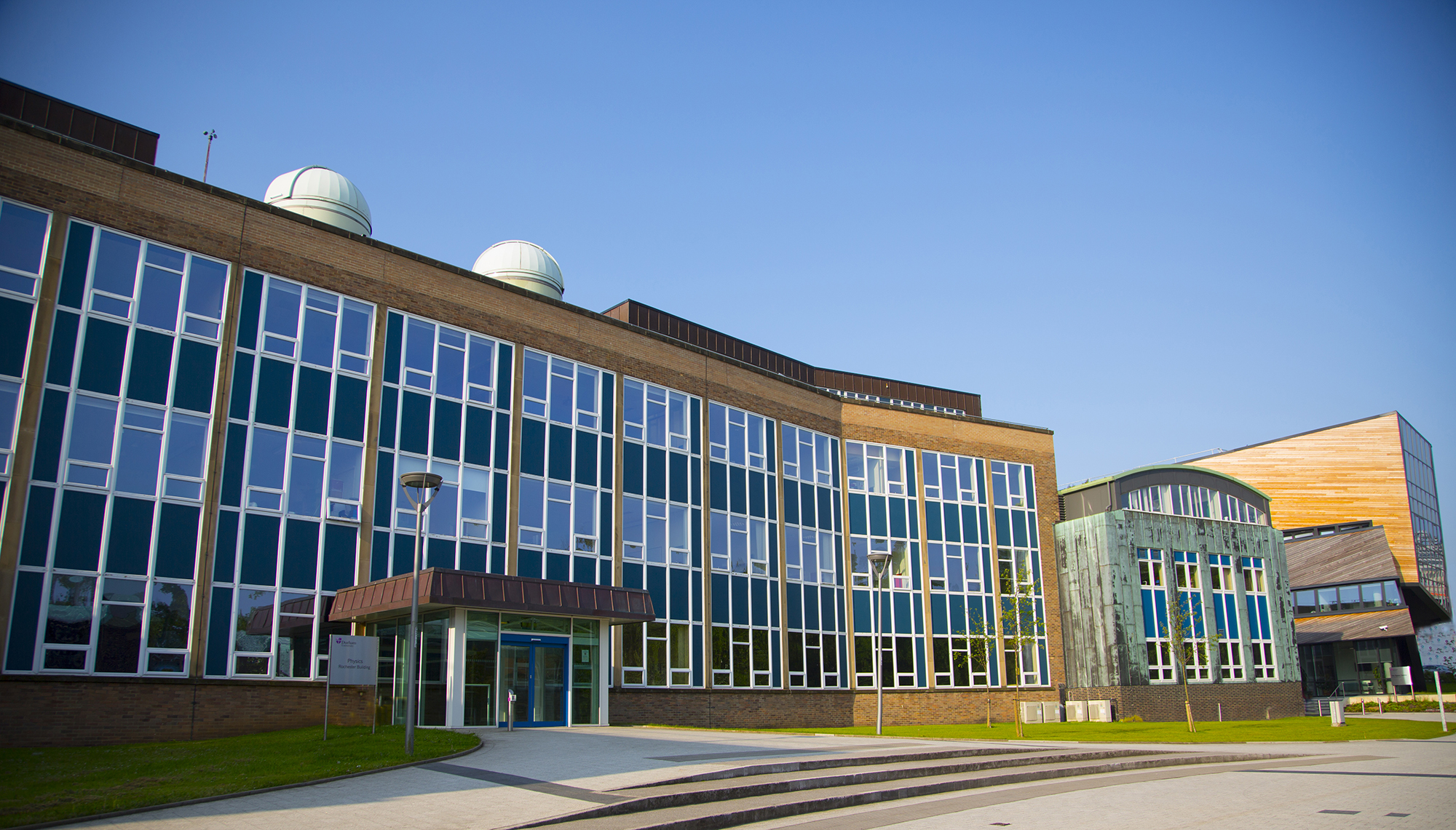
Our history
2024 marked 100 years of the Department of Science in Durham University, years that have seen the service of thirteen different Heads of Physics, hundreds of staff and thousands of students. To celebrate this milestone, you can now discover the history of Physics at Durham through the centuries.
From Temple Chevallier to the researchers of today, scroll through our timeline and meet some of the key figures from our history. Watch as some of our most influential academics from past and present talk about their experiences of Durham through the years. Learn about the buildings that have shaped our history, from the creation of the Observatory in the 1800s to the first dedicated building for Physics in the late 1950s, to our major investment in Astronomy going forward.
/prod01/prodbucket01/media/durham-university/departments-/physics/equality-and-diversity/Royal-Society-Flags-Group.jpeg)

Look Closer at the Faculty of Science
Whether it’s our world-leading research that seeks to empower and inspire, our commitment to educational excellence across eight academic departments, or our focus on the next generation of scientists through our ground breaking science outreach and engagement. We push forward, break down barriers, asking the big questions and getting answers. Watch our short video to find out why there’s more to science at Durham than meets the eye.
/prod01/prodbucket01/media/durham-university/departments-/physics/equality-and-diversity/Royal-Society-Flags-Group.jpeg)
/prod01/prodbucket01/media/durham-university/departments-/physics/staff/VT2A9495-2826X2018.jpeg)
/prod01/prodbucket01/media/durham-university/departments-/physics/telescopes/21AprilC.jpg)
/prod01/prodbucket01/media/durham-university/departments-/physics/buildings/Studio-Libeskind_The-Ogden-Centre_Durham-University_-%C3%82Hufton-Crow_026-3429X2337.jpg)
/prod01/prodbucket01/media/durham-university/departments-/physics/buildings/Ogden-1.jpg)
Open Days & Visits
We can offer personal tours of the Physics Department by arrangement, in addition to the University’s standard open day offerings. to discuss a department tour, please see ‘Arrange a personal tour’ below.
Experience Durham by arranging a personal tour
Arrange to have a personal tour of our department buildings and facilities, meet departmental staff and get a feel for what it would be like to study here.
Student updates
-
What it's been like studying Physics
3rd year Physics student Jack reflects on his studies during the pandemic
-
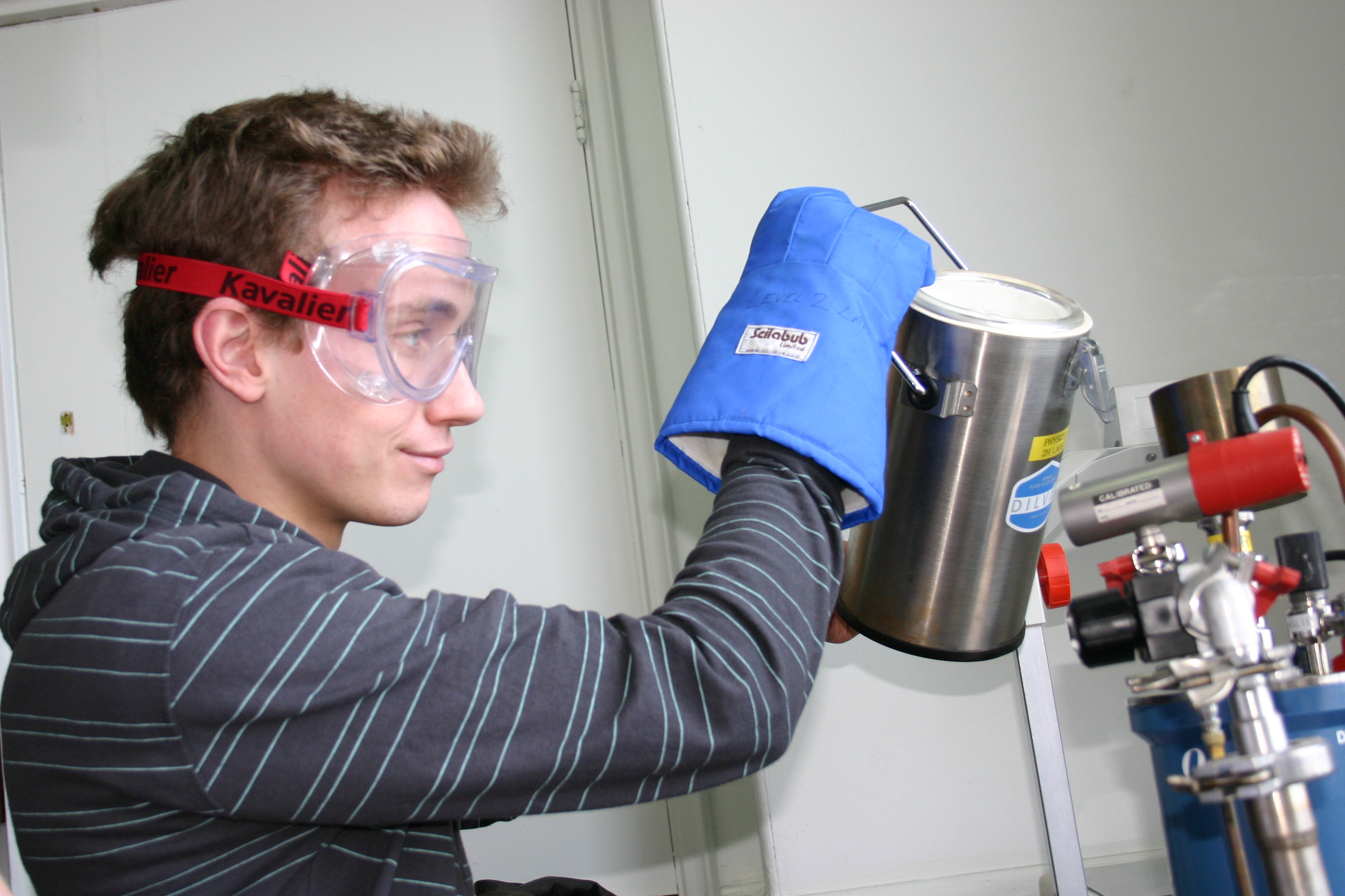
Day in the life of a 3rd year Physics student: My Industrial Project
Physics student Gabriel tells us about his Team Project module at Durham
/prod01/prodbucket01/media/durham-university/departments-/physics/buildings/PhysicsBuilding.jpg)
/prod01/prodbucket01/media/durham-university/departments-/physics/teaching-labs/IMG_3659.jpeg)
What it's been like studying Physics
3rd year Physics student Jack reflects on his studies during the pandemic
Day in the life of a 3rd year Physics student: My Industrial Project
Physics student Gabriel tells us about his Team Project module at Durham
Get in touch
Contact us to find out more about our department.
Department of Physics
Durham University
Lower Mountjoy
South Road
Durham
DH1 3LE
United Kingdom
Questions about studying here?
Check out our list of FAQs or submit an enquiry form.
Your Durham prospectus
Order your personalised prospectus and College guide here.