/prod01/prodbucket01/media/durham-university/departments-/physics/teaching-labs/VT2A9034-1998X733.jpeg)
LINEARISING DATA:
You may find that sometimes it is more convenient or convincing to show a linear relationship in your graphs, whereby the y values are directly proportional to the x values. For non-linear data it is necessary to first linearise it. This may be useful when dealing with acceleration due to gravity, as seen in the figures below, or for exponential decay.
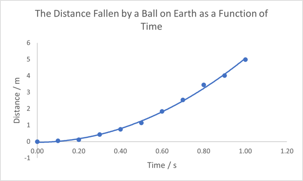
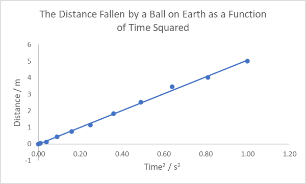
As shown in the figures above, plotting the linearised data clearly shows the x2 power law as you will have seen from the equations of motion for constant acceleration (or “SUVAT” equations). It is worth noting that if the data presented above were to deviate (even slightly) from this power law, the linearised data would show this more clearly, since the straight line would not be followed.
If you are unsure how to plot graphs like those seen above in Excel, you can see our Excel guide to graphs or our guide to creating trendlines (see 'other tips for Excel' page).