Poisson Distribution

Introduction

The Poisson distribution is a special case of the binomial distribution that it models discrete events. It expresses the probability of a number of relatively rare events occurring in a fixed time if these events occur with a known average rate, and are independent of the time since the last event.

In summary, the conditions under which a Poisson distribution holds are when:

counts are of rare events
all events are independent
average rate does not change over the period of interest

In physics, these conditions normally occur when we are dealing with counting – especially radioactive decay, or photon counting using a Geiger tube.

Unlike the normal or binomial distributions the only parameter we need to define is the average rate, or the mean of the distribution, for which NÌ„, or λ, are often used. The Poisson probability distribution is a single-parameter function which allows us to find the probability that there are exactly x occurrences (x being a non-negative integer, x = 0, 1, 2, ...). It is defined as

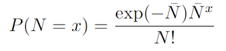
where NÌ„ is a positive number (not necessarily an integer) equal to the mean. As in the case for the Gaussian distribution we can find the mean and the standard deviation of the Poisson probability function. The average count rate, or mean, is NÌ„. As the function is only defined by one variable, it may not be surprising to find that the standard deviation is also related to the mean. The standard deviation of a Poisson distribution is simply the square root of the mean.

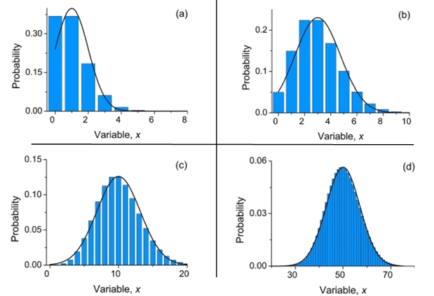
Fig. 1: The evolution of the Poisson distribution as the mean increases. The Gaussian distribution as a function of the continuous variable x is superimposed.

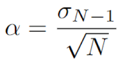
Standard Error

The standard error for poisson counting is the square root of the number of counts. I.e.

Using Excel

Excel can make calculations using equation 1 for us. To illustrate this, lets use an example. This example was taken from page 30, example 3.4.1 in Measurements and their Uncertainties, Ifan G. Hughes and Thomas P.A. Hase [link required].

"A safety procedure at a nuclear power plant stops the nuclear reactions in the core if the background radiation level exceeds 13 counts per minute. In a random sample, the total number of counts recorded in 10 hours was 1980. What is the count rate per minute and its error? What is the probability that during a random one-minute interval 13 counts will be recorded? What is the probability that the safety system will trip?"

We are going to use this example to show how excel can be used to make this problem simpler. A spreadsheet [link required] has already been prepared for you with the relevant data inputted.

By now, you should be able to calculate the mean and error by yourself, so we will focus on the poisson distribution calculations.

Fig. 2: Screenshot of a calculation involving the non-cumulative Poisson Distribution.

However, this is not the answer to the problem. We need to calculate the probability that the count rate would reach 13 or higher. To take this into account, we need to calculate the probability using a cumulative Poisson Distribution. This will calculate the probability that our variable is less than or equal to the inputted value.

Fig. 2: Screenshot of a calculation involving the cumulative Poisson Distribution.

Note that we were considering higher than 13 counts per minute, not less than. Hence we have to work out the probability of the reactor not exceeding 13 counts per minute and removing that from 1.

So why not use a calculator instead?

There are two main reasons for this

The cumulative Poisson calculation would have been very lengthy
If you want to change any of the starting numbers, the resulting calculations will change automatically. You don't have to start from scratch!

The second point is the most important. Regularly in your experiments you'll find that you'll only have to change one or two starting variables to a calculation, setting up a spreadsheet to do this easily saves a lot of time!